Static Compressive Object Tracking

Introduction

High resolution video for object tracking is a demanding application that requires expensive hardware and significant bandwidth to transmit. However if one is interested in estimating the location of moving objects rather than reconstructing the entire object scene, the information content in the signal-of-interest is relatively low.

The Static Compressive Optical Undersampled Tracking (SCOUT) camera is cool prototype camera developed by several researchers and myself to reduce the size, weight, and cost associated with high resolution tracking.

The goal of the camera is to capture low spatial resolution images and then in post-processing reconstruct the high-resolution object location. Certainly this seems counter-intuitive to traditional camera motion tracking, which cannot outperform the Nyquist sampling theorem.

However, using a signal processing technique called compressive sensing which utilizes the sparsity of the signal, one can significantly reduce the number of samples in the measurements.

How SCOUT Works

The SCOUT system takes measurements that are both compressive and multiplexed: The number of measurements is less than the number of scene locations, and each measurement must contain information about many scene locations. In this architecture, the number of measurements is the number of pixels in the CCD. Intuitively this means that the system matrix must exhibit a many-to-few mapping from scene locations to CCD pixels.

In this architecture the multiplexing occurs in the spatial domain by mapping multiple object scene locations to only a few detector pixels. To accomplish this, we created a structured blur. This blur allows the light from a single object point to be spread to several pixels on the CCD. The most straightforward way to achieve a blur is by defocusing the image so that the PSF is broad, spanning many CCD pixels. Since the number of CCD pixels are less than the object scene resolution, the measurement is compressive.

Defocus significantly reduces contrast of high spatial frequencies, so the measurements will be poorly conditioned for reconstruction. Therefore, we created high-frequency structure in the PSF by using two pseudo-random binary occlusion masks. Each mask is placed at different positions between the lens and the sensor. The separation between masks results in a spatially varying point-spread function.

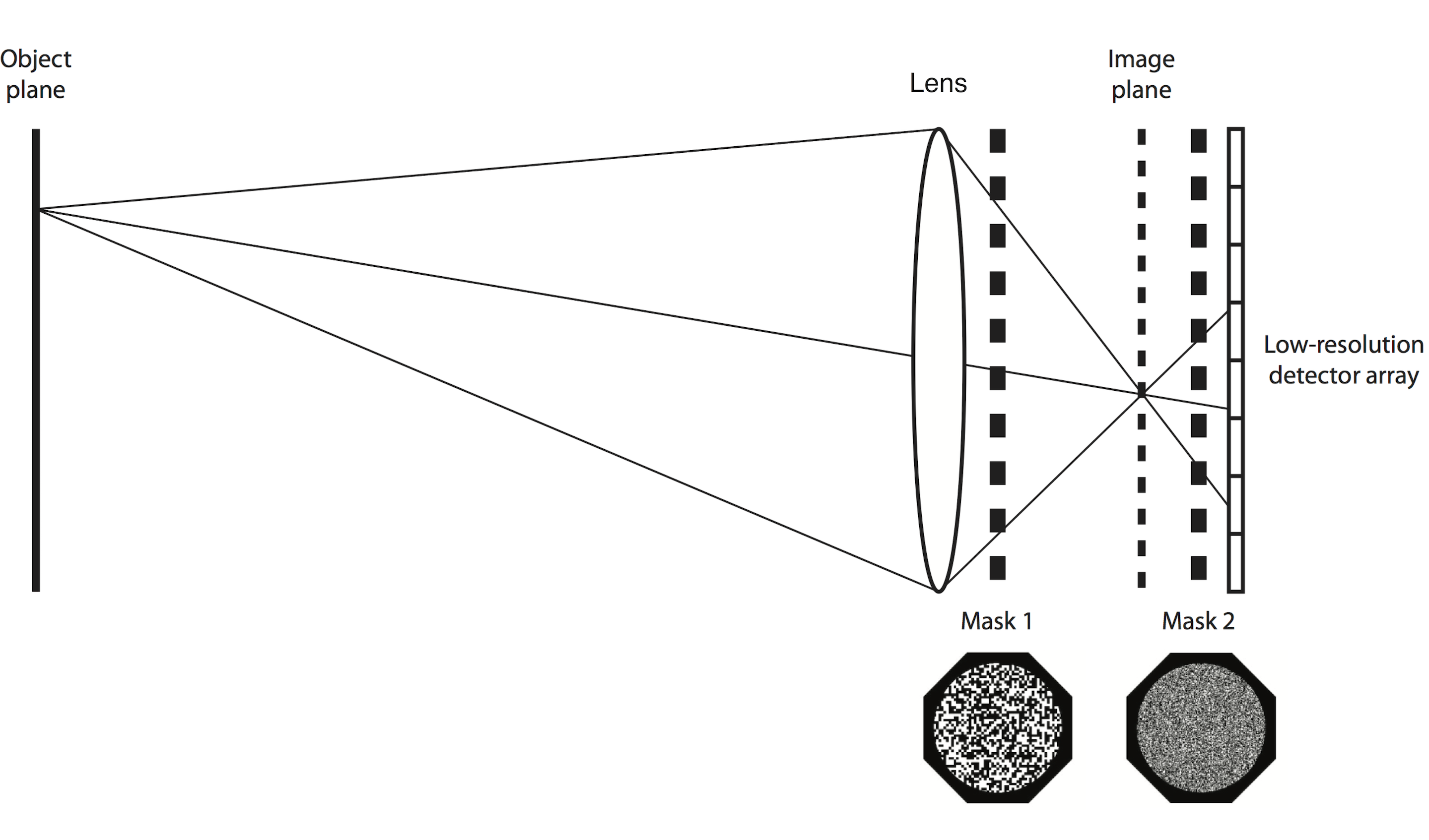
The architecture of the compressive object tracking camera is shown in the figure above. We use a low resolution image sensor which is placed at some distance away from the image plane, creating an intentional defocus. This produces a large PSF. There are two amplitude masks, which we created by using a laser printer on a transparency. The pattern of each amplitude mask is random. The first mask is placed adjacent to the lens and the second mask is placed near the CCD.

As with many linear computational sensing architectures, the forward model is written in the form

\[\mathbf{g} = \mathbf{H} \mathbf{f} + \mathbf{e}\]

where $\mathbf{f}$ is the discrete representation of the object signal-of-interest, $\mathbf{g}$ is the measurement, $\mathbf{H}$ is the matrix which describes mapping of the object to the measurement, and $\mathbf{e}$ is the noise at each measurement. In this situation the signal-of-interest is actually the difference between two subsequent object scenes (frames) $\Delta \mathbf{f}$:

\[\mathbf{g}_{k} = \mathbf{H} \mathbf{f}_{k} + \mathbf{e}_{k}\] \[\mathbf{g}_{k+1} = \mathbf{H} \mathbf{f}_{k+1} + \mathbf{e}_{k+1}\]

Where the subscripts represent the $k^{th}$ readout from the CCD.

\[\Delta \mathbf{g} = \mathbf{g}_{k+1} - \mathbf{g}_{k} = \mathbf{H} \{ \mathbf{f}_{k+1} - \mathbf{f}_{k} \} + \mathbf{e}_{k+1} - \mathbf{e}_{k}\]

so the forward model can be written as

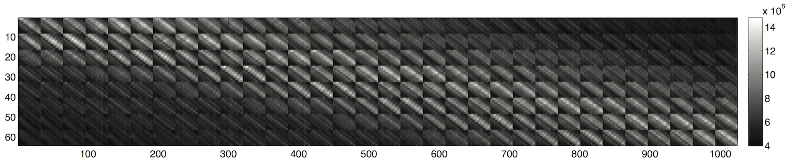
\[\Delta \mathbf{g} = \mathbf{H} \Delta \mathbf{f} + \Delta \mathbf{e}\]

In this equation, the 2-dimensional difference frame and object scene have a resolution of $R_x \times R_y$ elements, and are lexicographically reordered into a $N \times 1$ column vector, $\Delta \mathbf{f}$ and $\mathbf{f}$. Similarly, the difference measurement and measurement $\Delta \mathbf{g}$ and $\mathbf{g}$ are $N_m \times 1$ vectors representing a 2-dimensional CCD readout with a $r_x \times r_y$ matrix which represents the low resolution measurement. The detector noise is represented by the $N_m \times 1$ vector $\mathbf{e}$. The system matrix $\mathbf{H}$ is thus an $N_m \times N$ matrix, where $N_m \ll N$ in order to the system to be considered compressive. The $n^{th}$ column of the matrix is the PSF of the $n^{th}$ location in the object scene. The resulting system matrix $\mathbf{H}$ demonstrates that the SCOUT is a spatially variant optical system and presents a block structure:

Optimizing the SCOUT design

While the SCOUT lacks the ability to implement arbitrary measurement codes, we are able to adjust various physical parameters of the system such as defocus distance and mask fill factor to minimize reconstruction error. Adjusting each parameter in the actual prototype requires too much time, a more practical approach is to simulate the SCOUT architecture. In this section, I will discuss the simulation and define a metric that we used to evaluate different design parameters of the SCOUT without the need to reconstruct the difference frames.

We developed a paraxial ray based simulation for the SCOUT. The simulation allows us to model the effects on the measurement as light travels through the lens and two masks and onto the detector plane. The lens is modeled as a single thin lens with transmittance function $t_f$ and the two masks have transmittance functions $t_1$ and $t_2$. From calibration measurements, the mask has a transmittances of $0$ where the mask is black and $0.88$ where the mask is clear. The lateral magnification of the scene and the two masks is calculated using similar triangles.

A simulated calibration occurs, in other words the simulation records the $r_x \times r_y$ PSF from each scene location in order to obtain the system matrix $\mathbf{H}$. Once $\mathbf{H}$ is known, we use it to simulate the low resolution measurements, $\mathbf{g}$, of the higher resolution scenes, $\mathbf{f}$. Subsequent simulated measurements are subtracted to find $\Delta \mathbf{g}$. We also did not add any noise.

Quantifying Reconstruction Error:

The Mean Squared Error (MSE) error metric is not suitable for this application because it weights all errors equally. For the task of motion tracking, I classify errors into three types. A false positive occurs when the estimate shows an object where there is none. A false negative occurs when the estimate fails to show an object where one exists. As shift error occurs when an object is being tracked but appears in the wrong location. We developed a custom tracking error metric that weighs false negatives and false positives more than shift errors. This is because false negatives and false positives indicate a serious failure in the motion tracking task, while shift errors are less serious. I define tracking error as

\[P = \frac{ \left| \mathbf{a} \otimes \mathbf{\epsilon} \right| }{ 2N_{mv} }\]

where

\[\mathbf{a} = \begin{bmatrix} 1/9 & 1/9 & 1/9 \\ 1/9 & 1/9 & 1/9 \\ 1/9 & 1/9 & 1/9 \end{bmatrix}\]

where the error $\mathbf{\epsilon}$ is the difference between the true and reconstructed difference frames

\[\mathbf{\epsilon} = \Delta \mathbf{f} - \Delta \hat{ \mathbf {f} }\]

and $N_{\text{mv}}$ is the number of movers in the scene. To reduce the penalty for one-pixel shift errors, the error frame is convolved with a three pixel averaging kernel $\mathbf{a}$. The absolute value is taken in order to count positive and negative errors equally, and the error is divided by $2N_{mv}$ to make the metric independent of the number of movers.

Optimizing Optical System Parameters:

Now that I have explained the simulation and the custom error metric for tracking, I can finally begin to discuss how we optimized some of the parameters to reduce the reconstruction error. Both the simulation and experimental study demonstrates a relationship between mask position and pitch: the tracking error is very sensitive to the \emph{projected} mask pitch on the CCD. Furthermore, increasing the mask seperation reduced tracking error, generating a highly space-variant PSF. With these observations in mind, we focus our study on the mask pitches ($p_1$, $p_2$) as well as the defocus distance $d_{im}$.

A brute force search, reconstructing at each step is computationally intensive. I wanted a simple to compute metric which can predict tracking error. So we developed a custom metric inspired by the coherence parameter from the compressive sensing community. We created a customized coherence parameter $\mu$,

\[\mu = \max{\left| \langle h_i, h_j \rangle \right|} ; \qquad i \neq j\]

which is the maximum absolute value of the inner product between unique columns $h_i$ and $h_j$ of $\mathbf{H}$. The columns are unnormalized because their relative magnitude is related to the physical light throughput.

Notice that although system matrices with nearly pairwise orthogonal columns will result in small coherence values, system matrices with numerically small entries can accomplish the same. Optimizing $\mathbf{H}$ for minimum coherence would drive total system throughput down. To eliminate this effect we normalized $$\mathbf{H}$:

\[\mathbf{H}_{norm} = \frac{ \mathbf{H} }{ \sum_{m = 1}^{N_m} \sum_{n = 1}^{N} h_{m,n} }\]

where $N_m$ and $N$ are the total number of rows and columns in the system matrix. Physically, this normalization represents division by the sum of each PSF’s light throughput. The coherence of a system matrix normalized in this way cannot be biased by reducing throughput. One consequence of this normalization is that mask fill factor cannot be optimized.

The simulations demonstrate the viability of the architecture and provide an efficient way to optimize most architecture parameter values using the simulated system matrix coherence. Mask throughput cannot currently be optimized because the custom coherence metric is normalized by full system throughput. The problem of finding optimal mask throughput warrants further investigation.

Experimental Results:

These are actual experimental results:

(a) The high res ground truth image of the past scene. This is not measured.

(b) The high res ground truth image of the current scene. This is not measured.

(d) The low res measured difference image from the camera. This is the data is sent to the compressive sensing algorithm.

(e) The reconstructed high res difference image.