Designing a Cooke Triplet

The Cooke Triplet is the first and simplest design form that is capable of correcting all the first- and third-order aberrations over a medium field-of-view [1]. The Cooke Triplet consists of three elements. The two elements on the outside are positive crowns and the middle element is a negative flint. The aperture stop is located either in front of the middle element or behind it.

Inspired by my Lens Design class homework [2], in this post I will walk through the procedure for designing a Cooke Triplet from scratch using first-order thin lens calculations, then optimizing it with real thicknesses in Zemax OpticStudio.

System Specs

The desired focal length of the system is \(f_E = 50 \text{ mm}\) therefore the power is \(\phi_{E} = 0.02 \text{ mm}^{-1}\).

Glass: N-SK16 (\(n_d\)=1.620410, V=60.323649) and N-SF2 glass (\(n_d\)=1.647690, V=33.820209).

Field angles: \(0^{\circ}, 10^{\circ}, 20^{\circ}\).

Wavelengths: (587.56 nm), F (486.13 nm), and C (656.27 nm) wavelengths.

Paraxial F/#: 4

The Starting Point

The starting point of the first-order design is to imagine the Cooke Triplet as a pair of air spaced achromatic doublets. The second achromatic doublet (Doublet 2) has exactly the same radii of curvatures as the first except with opposite signs.

The Gaussian reduction equation for total power of two elements is:

\[\phi_{E} = \phi_1 + \phi_2 - \phi_1 \phi_2 \tau\]

Where \(\tau = t / n\) is the reduced thickness, \(t\) is the physical thickness, and \(n\) is the index of refraction of the medium between the two elements.

If we approximate the airspace as zero \(\tau \approx 0\) and assume Doublet 1 & 2 have the same focal length, then each doublet has half the power of the total system power:

\[\phi_{E} = \phi_1 + \phi_2 \quad \text{ such that } \quad \phi_1 = \phi_2\]

Thus the power of each air spaced achromatic doublet is:

\[\phi_1 = \phi_2 = 0.01 \text{ mm}^{-1}\]

Now we need to solve for the powers of the positive and negative elements of one achromatic doublet. Again assume no air gap. Using the Gaussian reduction equation again, the power of the positive lens plus the power of the negative lens is the power of the doublet:

\[\phi_{11} + \phi_{12} = 0.01 \text{ mm}^{-1}\]

For an achromatic doublet the following formula must hold to put the F and C wavelengths at the same focus [3]:

\[\frac{\phi_{11}}{V_1} + \frac{\phi_{12}}{V_2} = 0\]

Since we have two equations and two unknowns we can solve for the power of the positive and negative element:

\[\phi_{11} = 0.0227606 \text{ mm}^{-1}\] \[\phi_{12} = -0.012760 \text{ mm}^{-1}\]

We can use the thin lens equations to solve for the radii of each element in the achromatic doublet:

\[\left( n_{d2} - 1 \right) \left( C_3 - C_4 \right) = \phi_{12}\] \[\left( n_{d1} - 1 \right) \left( C_1 - C_2 \right) = \phi_{11}\]

Since the fourth surface is flat:

\[C_4 = 0\]

Assume the second and third have the same radii of curvature:

\[C_2 = C_3\]

Which produces

\[C_1 = 0.016984 \text{ mm}^{-1} \text{ and } R_1 = 58.7668 \text{ mm}\] \[C_2 = -0.019701 \text{ mm}^{-1} \text{ and } R_2 = -50.7567 \text{ mm}\] \[C_3 = -0.019701 \text{ mm}^{-1} \text{ and } R_3 = -50.7567 \text{ mm}\] \[C_4 = 0.0 \text{ mm}^{-1} \text{ and } R_4 = \infty \text{ mm}\]

The second achromatic doublet will have the same radii with opposite signs.

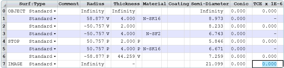
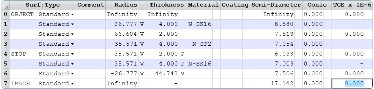
\[C_5 = 0.0 \text{ mm}^{-1} \text{ and } R_5 = \infty \text{ mm}\] \[C_6 = 0.019701 \text{ mm}^{-1} \text{ and } R_6 = 50.7567 \text{ mm}\] \[C_7 = 0.019701 \text{ mm}^{-1} \text{ and } R_7 = 50.7567 \text{ mm}\] \[C_8 = -0.016984 \text{ mm}^{-1} \text{ and } R_8 = -58.7668 \text{ mm}\]

We input these into Zemax without any airspaces, which collapses into five surfaces, the Lens Data editor now looks like:

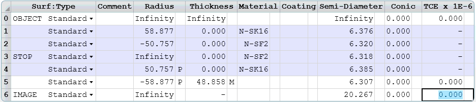
Notice that next to the radius data for surface 4 and 5 there is a “P”. This is to signify a “Pick-Up Solve”. Pick-Up solves are useful for constraining the parameter to be some scalar multiple of another parameter at another surface. In this case, I am using the pick-up solve to make the radii equal but opposite.

Next to the thickness for surface 5 there is a “M”. This is to signify a “Marginal Ray solve”. The marginal ray solve is used to set the thickness from the last optical surface to the image plane so the marginal ray crosses the optical axis at the image plane, thus placing the image plane at the paraxial image location.

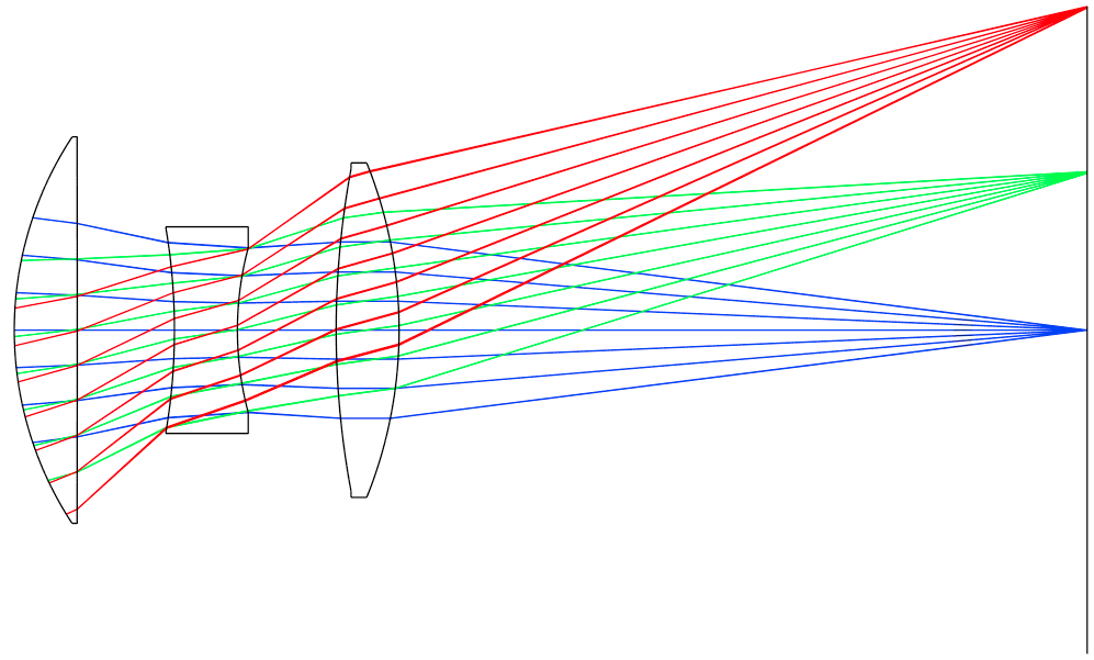
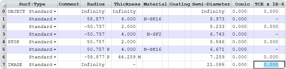
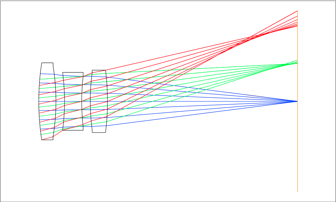
We are now at the paraxial thin-lens starting point for the Cooke Triplet. Surface 3 is not useful since rays are going from and into the same glass, so we will delete that. Then we will go ahead and add 4 mm of thickness to the elements and 2 mm of thickness to the airspaces.

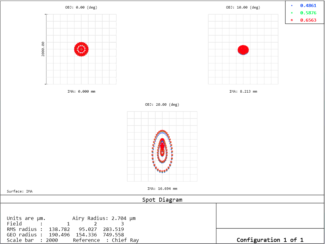
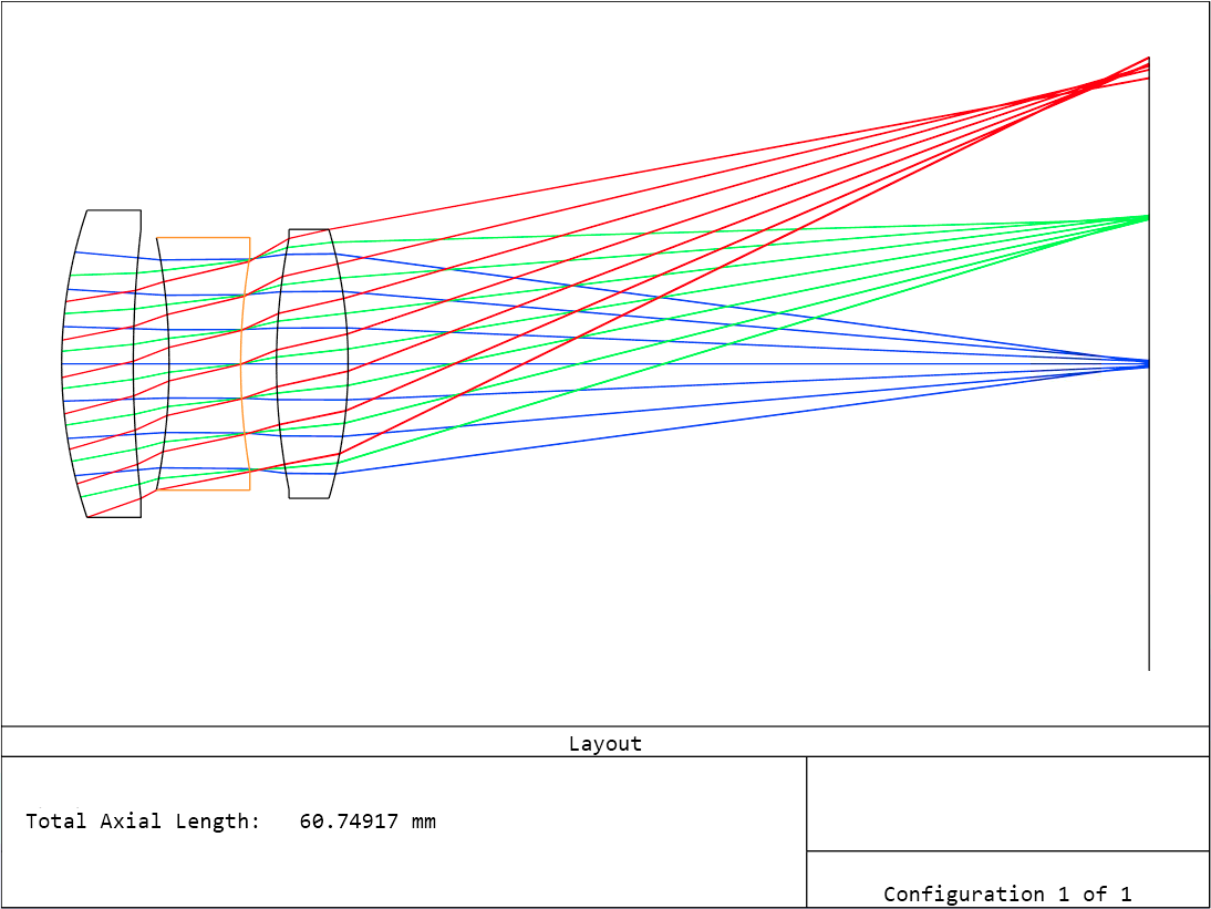
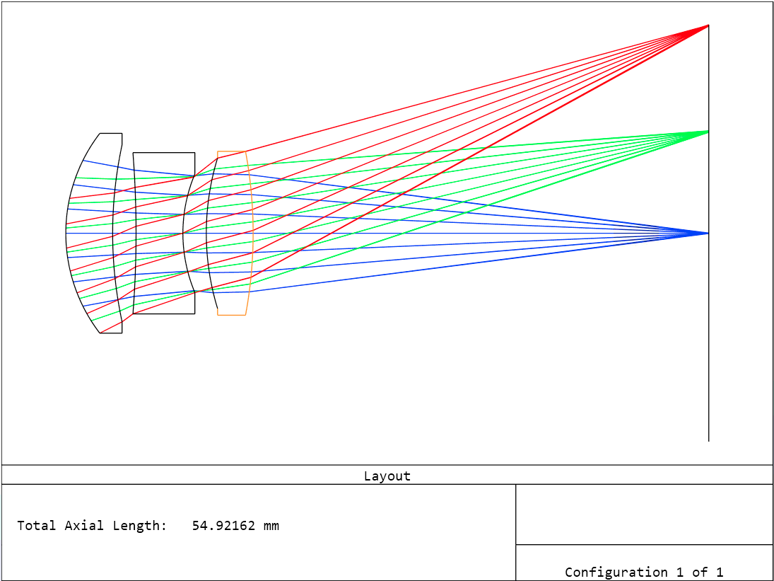
The 2D Layout shown below shows significant coma aberration in the caustic of the off-axis fields.

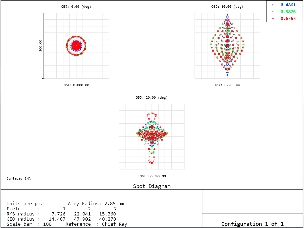
This spot diagram confirms this.

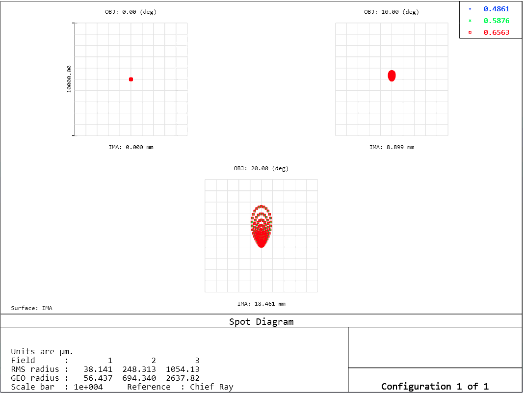
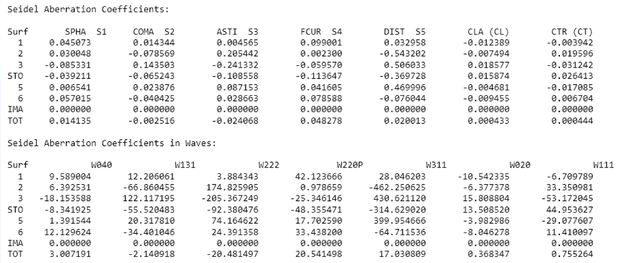
While specific aberrations are difficult to quantify from the spot diagram, Zemax calculates specific Siedel coefficients and converts them in terms of wavefront error with units of waves.

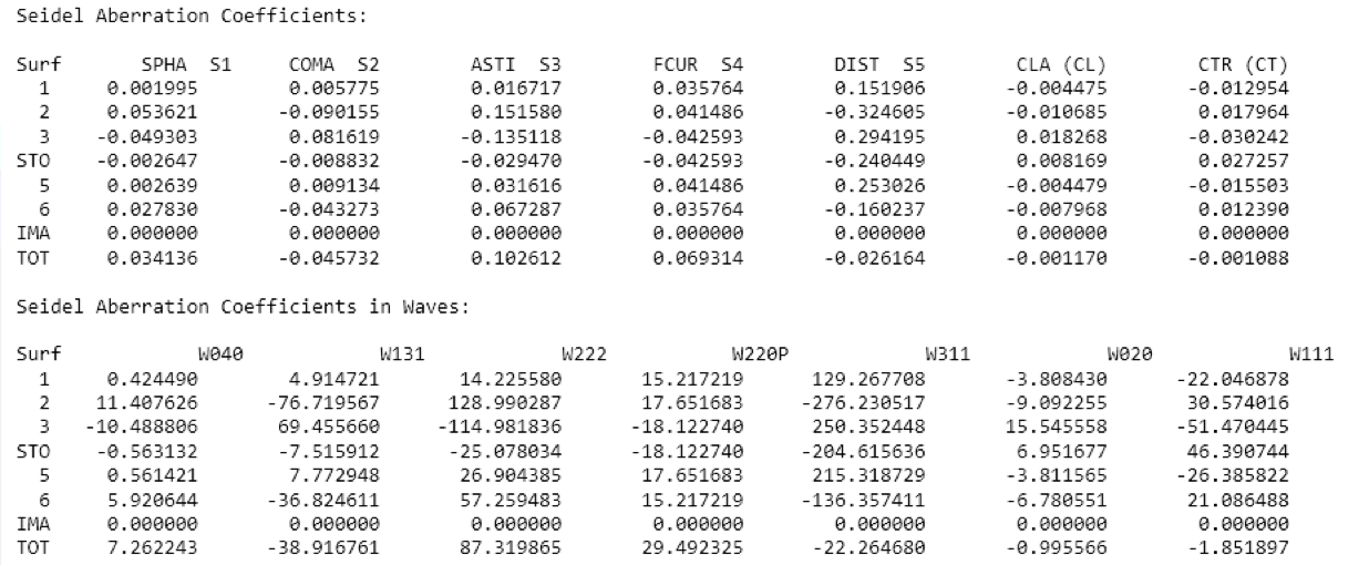
This shows that astigmatism is actually the most dominant aberration with 87.3 waves of wavefront error shown by the \(W_{222}\) term. Coma is the second most dominant with -38.9 waves of error as shown by the \(W_{131}\) term. Remember this is just a listing of the third-order aberrations.

Initial Optimization Iteration

We create a merit function using the Zemax Optimization Wizard with attempts to minimize the root-mean-squared (RMS) spot size radius calculated from the centroid, with 3 rings and 6 arms. We also insert an optimization operand, EFFL, to control the effective focal length of 50 mm.

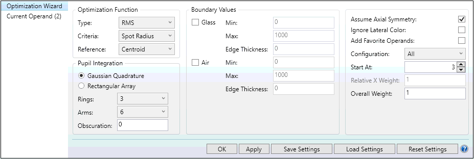
The three unconstrained radii and the lens to image plane thickness are set as optimization variables:

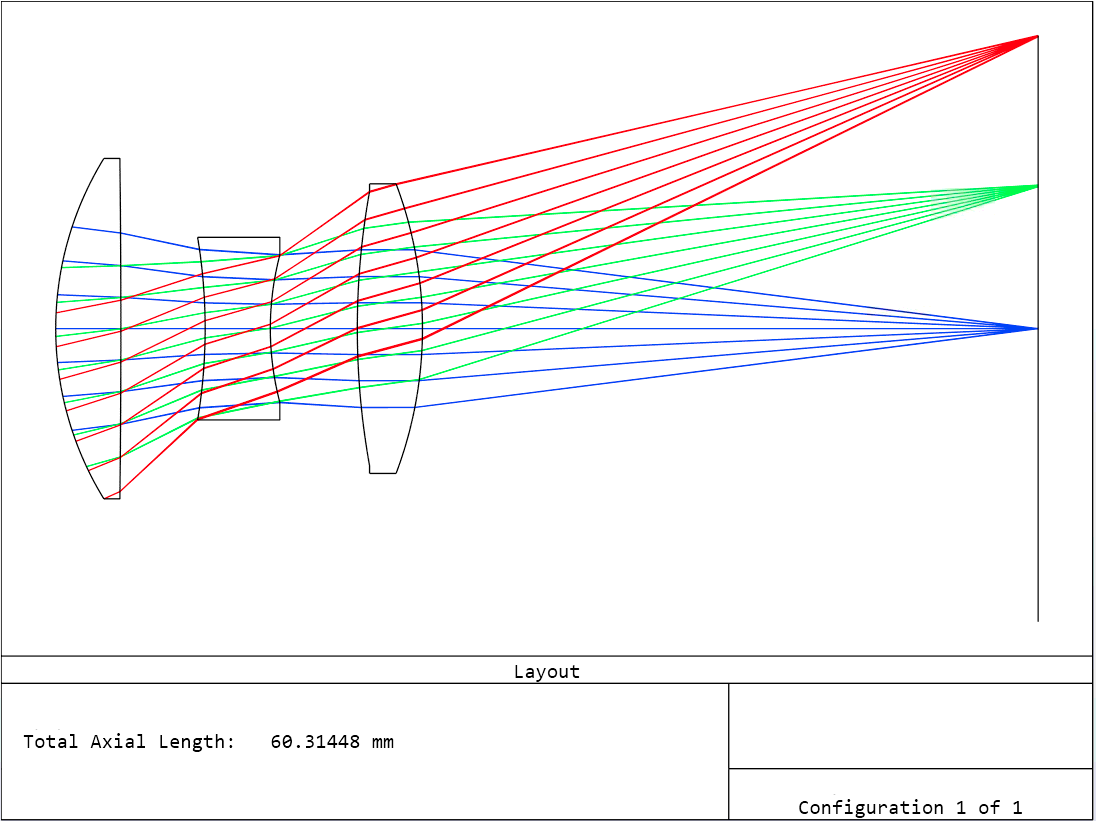
After performing the optimization the off-axis spot size has been reduced by a factor of 3.3.

The off-axis field’s caustic also shows reduced coma aberrtion. While spherical aberration dominates the on-axis field.

The next step is to allow all the curvatures to be optimization variables

and reoptimize.

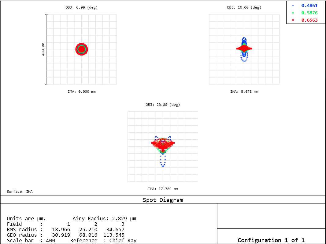
There is significant improvement in the spot diagram for the \(20^{\circ}\) field!

Just by inspection of the layout, the caustic for both the on-axis and off-axis seem to be free of coma and spherical which plauged the us earlier.

Finally we allow the two air spacings to be optimization variables and reoptimize.

It is possible to correct all seven first- and third-order aberrations exactly to zero in a Cooke Triplet, however in practice this is not done. Third-order aberrations are non-zero to balance the higher-order aberrations. This cancellation is not perfect either, so, Cooke Triplets are usually restricted to applications requiring only moderate speed and field coverage [4].

We are not yet diffraction limited and there are certainly more steps one can take but we stop here. Any significant improvement would most likely involve lens splitting, glass choice, and/or aspheres. As one can see in the design, using only spherical elements with relative common glass choice, it performs well on- and off-axis.

The Cooke Triple holds a special place in optical design history, while they have been replaced in modern camera objectives by more complex designs, the Cooke Triplet maybe a good choice when simplicity, cost, ruggedness, and good performance over a medium field-of-view are desired. In the near future, I will write a blog post that discusses how the Cooke Triplet actually accomplishes the correction of the first- and third-order aberrations using the formalism of paraxial ray tracing and Siedel coefficients.

1. J. Bentley and C. Olson, “Field Guide To Lens Design,” SPIE Press (2012)
2. D. Marks, “ECE 676 Lens Design Homework 4”, Duke University 2013
3. J. Greivenkamp, “Field Guide To Geometrical Optics,” SPIE Press
4. W. J. Smith, “Modern Optical Engineering, second edition”, Tata McGraw-Hill Education